Time series analysis
Components of a time series
- Seasonality/periodicity
- Stationarity
- Autocorrelation
Stochastic process
OK, so I was considering what's a Dirichlet distribution and what's a categorical, because I don't know what a slice from the area chart of activities over 24 hours (you know the one) would be. I guess categorical, not Dirichlet, because it's a rigid group of probabilities, like the Bernoulli
Good visualization of Bernoulli: gave me an "aha".

Then onwards to the categorical. Look!

This is a regular Cartesian 3-D coordinate system, so you're meant to see the triangle as standing slanted against the vertical axis. Make sense?
The entire triangle is not a categorical distribution; rather, the triangle is the space of all possible categorical distributions. One distribution would be a single point on it. A tuple of three p-values that add up to 1.
This triangle visualization is important, because now see the Dirichlet:
en.wikipedia.org/wiki/File:Dirichlet.pdf
Now let's backtrack to the Bernoulli and beta distributions to make sure you understand it. Does the beta make sense to you – are you fully clear on what the x and y axes represent?

At any point on the x-axis between 0 and 1, you have a tuple of two values p and (1-p). So, x = 0.3 represents the Bernoulli distribution where p = 0.3 and 1-p = 0.7. And the y-axis says how likely you are to observe this particular tuple. Yes, kind of a "probability of a probability"… Although x could represent any number-pair that has to add to 1 or some other given fixed sum.
But really, when you model a generative process as a Bernoulli of unknown parameters, it makes sense to have, as prior, a probability distribution over all possible Bernoulli distributions, so yes, a prob of a prob.
You might think p = 0.1 and 1-p = 0.9 is a likely description of the generative process behind some variable but the reversed pair is not, so for your beta prior you might set α = 2 and β = 5 (orange line here).
So that one area chart is a distribution of categoricals over time.
A distribution of Dirichlets over time would be like if we took one of those triangles and extrude it out like a Toblerone. If we imagine the white background as invisible, it might look like a blue snake in the midst of writhing around.
This led me to ask what a Dirichlet process is. Ok, first it's a stochastic process. Are they always over time? Of course not necessarily, but what exemplifies it as a process is there's usually some relation to "past" values or simply "neighboring values on one axis", that axis not being one of the parameters to the Dirichlet itself.
A simple stochastic process is the Bernoulli process, which you'll recognize as the coin-flip process. A sequence of iid rv where each rv takes values 0 or 1. There's no autocorrelation of any kind. We can still draw a contiguous line on a chart if we consider each draw of the process as the sum of all previous draws.
A random walk is similar. The simple random walk is like the coin-flip process, but the rv takes values of 1 or -1 instead of 1 or 0. Interestingly, it's kind of hard to define one on continuous time – normally the steps in the time t are discrete.
The Wiener process, historically also called the Brownian motion process, is based on the normal distribution instead of the Bernoulli. The size of each change is distributed per the Gaussian.

Apparently, the Wiener process is a member of several families of processes: Markov processes, Levy processes and Gaussian processes.
The Wiener is Markovian, really? This leads me to: what is a Markov process? Wikipedia and Google seem to treat the term as synonymous with a Markov chain.
Generally, "a Markov chain is a stochastic model describing a sequence of possible events in which the probability of each event depends only on the state attained in the previous event."
As with most processes, there is a distinction between discrete-time (DTMC) and continuous time (CTMC) Markov chains.
AR/MA
One of the simplest time series models is a Moving Average model. It predicts the next point as the mean of all past datapoints, end of story. The equation is as follows.
xt = μ
Actually I lied, that's just conceptual. You need a few more variables,
- εt-i ("error terms", how much a datapoint was off from μ at time t),
- θi,
- and one hyperparameter q which controls how high i goes (so how many datapoints back to look).
The MA(q) model:
node:internal/modules/cjs/loader:1228
throw err;
^
Error: Cannot find module 'katex'
Require stack:
- /home/kept/private-dotfiles/.config/emacs/texToMathML.js
at Module._resolveFilename (node:internal/modules/cjs/loader:1225:15)
at Module._load (node:internal/modules/cjs/loader:1051:27)
at Module.require (node:internal/modules/cjs/loader:1311:19)
at require (node:internal/modules/helpers:179:18)
at Object.
For I suspect archaic reasons, the q parameter is also called the "order" of the model. And with that we have revealed the jargon behind the classic time series models, MA(q), AR(p), ARMA(q, p) and ARIMA(q, d, p).
AR: Autoregressive MA: Moving Average ARMA: Autoregressive Moving Average ARIMA: Autoregressive Integrated Moving Average
Each of these time series models exist in different orders. E.g. MA(0), MA(1), MA(2), AR(0), AR(1), AR(2), ARMA(1, 2), ARIMA(1, 2, 3).
ARIMA(1, 0, 0) is AR(1).
ARIMA(0, 0, 1) is MA(1).
ARIMA(1, 0, 1) is ARMA(1, 1).
Others: ARIMAX, VARIMA, SARIMA, FARIMA/ARFIMA.
Given an ARIMA(p,d,q), if d>0 one can modle this as an ARMA by running an ARMA(p,q) after differencing the original series d times.
Before 1970, econometricians and time series analysts used vastly different methods to model a time series. Econometricians modeled time series are a standard linear regression with explanatory variables suggested by economic theory/intuition to explain the movements in time series data. They assumed that the time series being ‘nonstationary’ (growing overtime) had no effect on their empirical analysis. Time series analysts on the other hand ignored this traditional econometric analysis. They modeled a time series as a function of its past values. They worked around the problem of nonstationarity by differencing the data to make it stationary. Then, Clive Granger and Paul Newbold happened[1]. Econometricians were forced to pay attention to the methods of time series analysts, the most famous of which was the Box–Jenkins approach developed by George P Box and Gwilym Jenkins and published in their legendary monograph Time Series Analysis: Forecasting and Control[2] .
Box and Jenkins claimed (successfully) that nonstationary data can be made stationary by differencing the series.
Econometricians ignored the Box-Jenkins approach at first but were forced to pay attention to them when it ARIMA forecasts started consistently outperforming forecasts based on standard econometric modelling. The lack of sound economic theory behind the ARIMA was troubling for econometricians to accept. They responded by developing another class of models that incorporated auroregressive and moving average components of Box-Jenkins approach with the ‘explanatory variables’ approach of standard econometrics. The simplest of such models is the ARIMAX which is just an ARIMA with additional explanatory variables provided by economic theory.
ARIMA models are applied in some cases where data show evidence of non-stationarity, where an initial differencing step (corresponding to the "integrated" part of the model) can be applied one or more times to eliminate the non-stationarity.
The AR part of ARIMA indicates that the evolving variable of interest is regressed on its own lagged (i.e., prior) values. The MA part indicates that the regression error is actually a linear combination of error terms whose values occurred contemporaneously and at various times in the past.
VARIMA (Vector Autoregressive…) is for when you have multiple time series, then at each time point t you can think of it as having a vector of values.
Sometimes a seasonal effect is suspected in the model; in that case, it is generally considered better to use a SARIMA (seasonal ARIMA) model than to increase the order of the AR or MA parts of the model.
If the time-series is suspected to exhibit long-range dependence, then the d parameter may be allowed to have non-integer values in an autoregressive fractionally integrated moving average model, which is also called a Fractional ARIMA (FARIMA or ARFIMA) model.
The Hurst exponent is used as a measure of long-term memory of time series. It relates to the autocorrelations of the time series, and the rate at which these decrease as the lag between pairs of values increases.
Invertability of MA processes
Why do we care? We don't really. stats.stackexchange.com/questions/333802/why-do-we-care-if-an-ma-process-is-invertible
Difference between time series and survival analysis
Survival analysis: dataset looks like this, and each row concerns a separate individual.
| time to death |
|---|
| 20 |
| 23 |
| 2 |
| 10 |
| 22 |
| 21 |
Time series analysis: dataset looks like this, and the whole dataset is about a single individual.
| time | value of interest |
|---|---|
| 1 | 40 |
| 2 | 39 |
| 3 | 40 |
| 4 | 41 |
| 5 | 47 |
| 6 | 46 |
The Wiener process - "Brownian motion"
d<- tibble(x = rnorm(100),
           y = rnorm(100))
ggplot(aes(x, y)) + geom_point()
ts.plot(d$x)
ts.plot(d$y)
The higher the temperature, the more powerful movements.
- X(0) = 0
- independent and stationary increases
- X(t2 ) - X(t1) ∈ N(E[Δ t]= 0, σ \sqrt[t_2 - t_1])
- E[X(t)] = 0, γ(s,t) = σ min(s, t)
- Not derivable
Sampled wiener process
X(tn) = X(0) + ϕ1 + ϕ2 + … + ϕn = X(tn-1) + ϕn
X(t1) = X(0) + ϕ1
Discrete random walk!
The discrete "sampled process": X(tn) = X(tn-1) + ϕn where ϕn ∈ N(0, σe), which is Gaussian white noise.
Example: satellites Sputnik 1, 2, 3 triangulates a GPS user's position and introduces white noise, electronic warfare.
Random walk
{ ϕ1, ϕ2, …, ϕn } a sequence of independent identically distributed random variables E(ϕi) = 0
Cov(ϕi, ϕj) = 0 where i ≠ j, otherwise σ2e.
Yt = 0 + ϕ1, ϕ2, …, ϕt = ∑ ϕi
This is the same as running cumsum() in R.
- E(Y(t)) = E(∑ϕi) = ∑ E(ϕi) = 0 + 0 + 0 … 0 = 0, iow the expected value is a constant
- V(Y(t)) = V(∑ϕi) = ∑ V(ϕi) = V(ϕ1) + V(ϕ2) + … + V(ϕt) = = σ2e + σ2e + … + σ2e = tσ2e so the variance depends on t \implies not stationary
- γY(t, s) = (a t × s covariance matrix) = ∑ ∑ C(ϕi, ϕj) = t We said this is zero for all i ≠ j, so this is the same as V(Y(t)) i.e. tσ2e. Though if 1 ≤ s ≤ t, it is sσ2e!
Example:
node:internal/modules/cjs/loader:1228
throw err;
^
Error: Cannot find module 'katex'
Require stack:
- /home/kept/private-dotfiles/.config/emacs/texToMathML.js
at Module._resolveFilename (node:internal/modules/cjs/loader:1225:15)
at Module._load (node:internal/modules/cjs/loader:1051:27)
at Module.require (node:internal/modules/cjs/loader:1311:19)
at require (node:internal/modules/helpers:179:18)
at Object.
Strong autocorrelation here.
Characteristics of AR
A simple general model AR(p = 1): { Yt = Φ Yt-1 + ϕt, ϕt ∈ N(0, σe) }
What happens if Φ > 1, Φ = 0, |Φ| > 1, -1 < Φ < 0, 0 < Φ < 1 ??
- Φ = 0
- \implies Yt = ϕt, so just white noise unrelated to the past
- Φ > 1
- (for example) Φ = 2 means that Y2 = 2 Y1 + ϕ2 Y3 = 2 Y2 + ϕ3 and so on, it is explosive & non-stationary and eclipses the effect of ϕt (?)
- 0 < Φ < 1
- (for example) Φ = 0.9 means that Y1 = 0.9Y0 + ϕ1 Y2 = 0.9Y1 + ϕ2 the effect of previous values is continually being subdued
- -1 < Φ < 0
- (for example) Φ = -0.9 Y1 = -0.9Y0 + ϕ1 Y2 = -0.9(-0.9Y0) + ϕ2 It flips sign for every point. If the starting value is 4, it goes to -3.6, then 3.24 and so on, hugging the x-axis ever closer.
- |Φ| > 1
- (for example) Φ = -2 Like the case of Φ = 2, but it flips sign. So it gets further and further away from the x-axis.
Unevenly spaced time series
When analysts are presented with unevenly-spaced sensor data, they usually convert the unevenly-spaced data to a evenly-spaced time series by regular sampling or linear interpolation. This conversion helps get the data into a format that are used by the most common tools for time series analysis. In addition to the constraints on data size, this method also presents other practical challenges:
It is easy to make mistakes. Since evenly-spaced time series are usually stored without timestamps (in an array, along with the start time and time interval), it’s easy to use the wrong time units — conversions are notoriously error-prone — or mix up when the data was recorded. It encourages bloat. If you have data from several sources with different time resolution, the usual approach is to sample at the smallest time resolution. You can end up with a time series that is sampled every second from a sensor that samples every hour.
Beyond the practical challenges, there are technical reasons to be careful when converting unevenly-spaced data to regular time series including:
Data loss and dilution. You lose data that are closely spaced, and you add redundant data points when the data are too sparse.
Time information. The duration between each measurement can contain useful information about the data. For example, based on the frequency and duration of the light switching on or off, we can safely say that the second house is more likely to use an automated light switch than the first house.
Kalman Filter
Kalman filters are ideal for systems which are continuously changing. They have the advantage that they are light on memory (they don’t need to keep any history other than the previous state), and they are very fast, making them well suited for real time problems and embedded systems.
Let’s make a toy example: You’ve built a little robot that can wander around in the woods, and the robot needs to know exactly where it is so that it can navigate.
We’ll say our robot has a state node:internal/modules/cjs/loader:1228
throw err;
^
Error: Cannot find module 'katex'
Require stack:
- /home/kept/private-dotfiles/.config/emacs/texToMathML.js
at Module._resolveFilename (node:internal/modules/cjs/loader:1225:15)
at Module._load (node:internal/modules/cjs/loader:1051:27)
at Module.require (node:internal/modules/cjs/loader:1311:19)
at require (node:internal/modules/helpers:179:18)
at Object.
In our example it’s position and velocity, but it could be data about the amount of fluid in a tank, the temperature of a car engine, the position of a user’s finger on a touchpad, or any number of things you need to keep track of.
Our robot also has a GPS sensor, which is accurate to about 10 meters, which is good, but it needs to know its location more precisely than 10 meters. There are lots of gullies and cliffs in these woods, and if the robot is wrong by more than a few feet, it could fall off a cliff. So GPS by itself is not good enough.
We might also know something about how the robot moves: It knows the commands sent to the wheel motors, and its knows that if it’s headed in one direction and nothing interferes, at the next instant it will likely be further along that same direction. But of course it doesn’t know everything about its motion: It might be buffeted by the wind, the wheels might slip a little bit, or roll over bumpy terrain; so the amount the wheels have turned might not exactly represent how far the robot has actually traveled, and the prediction won’t be perfect.
- The GPS sensor tells us something about the state, but only indirectly, and with some uncertainty or inaccuracy.
- Our prediction tells us something about how the robot is moving, but only indirectly, and with some uncertainty or inaccuracy.
But if we use all the information available to us, can we get a better answer than either estimate would give us by itself?
We don’t know what the actual position and velocity are; there are a whole range of possible combinations of position and velocity that might be true, but some of them are more likely than others:
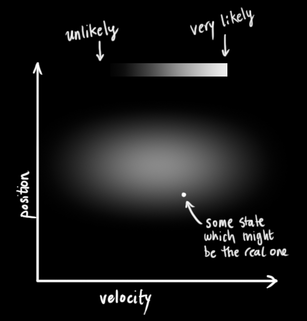

In the above picture, position and velocity are uncorrelated, which means that the state of one variable tells you nothing about what the other might be.
The example below shows something more interesting: Position and velocity are correlated. The likelihood of observing a particular position depends on what velocity you have:
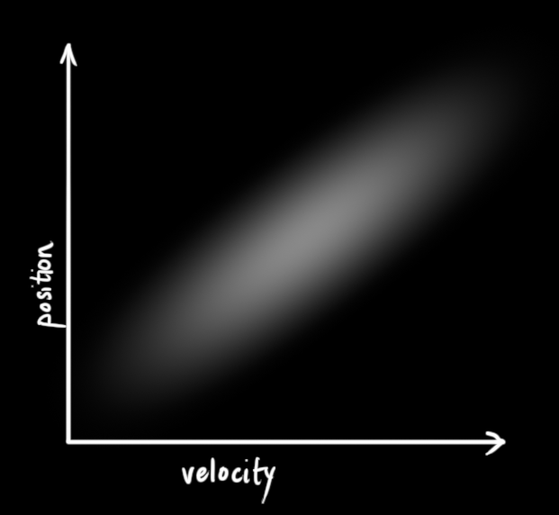
This kind of situation might arise if, for example, we are estimating a new position based on an old one. If our velocity was high, we probably moved farther, so our position will be more distant.
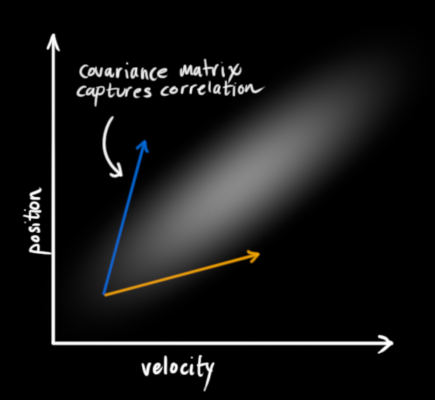
This correlation is captured by something called a covariance matrix. In short, each element of the matrix node:internal/modules/cjs/loader:1228
throw err;
^
Error: Cannot find module 'katex'
Require stack:
- /home/kept/private-dotfiles/.config/emacs/texToMathML.js
at Module._resolveFilename (node:internal/modules/cjs/loader:1225:15)
at Module._load (node:internal/modules/cjs/loader:1051:27)
at Module.require (node:internal/modules/cjs/loader:1311:19)
at require (node:internal/modules/helpers:179:18)
at Object.
Example dataset would be nice, so I can translate what guides tell me into something meaningful for me.
Dynamic linear models (DLM) are a special case of general state space models. Estimates for a DLM can be gotten by the famous Kalman filter.
ARMA models are a special case of state space models.
The Kalman filter and generalized variants are based on a hidden Markov model (HMM) where all latent and observed variables are continuous. So I guess you would not use it for a classification problem. Though apparently DuckDuckGo returns hits. yuyanwei.github.io/papers/kai2020orderingACCESS.pdf seems well written.
Correlation and covariance
- Cov(X, Y) is also written γX,Y(X,Y) and defined as E(XY) - E(X)E(Y).
- Corr(X, Y) is also written ρX,Y(X,Y).
Having only one subscript (CovX) makes it an autocovariance function. You may see it written the following way. Otherwise it is called cross-covariance.
node:internal/modules/cjs/loader:1228
throw err;
^
Error: Cannot find module 'katex'
Require stack:
- /home/kept/private-dotfiles/.config/emacs/texToMathML.js
at Module._resolveFilename (node:internal/modules/cjs/loader:1225:15)
at Module._load (node:internal/modules/cjs/loader:1051:27)
at Module.require (node:internal/modules/cjs/loader:1311:19)
at require (node:internal/modules/helpers:179:18)
at Object.
Having only one subscript (CorrX) makes it an autocorrelation function (ACF). Yoy may see it written the following way. Otherwise it is called cross-correlation.
node:internal/modules/cjs/loader:1228
throw err;
^
Error: Cannot find module 'katex'
Require stack:
- /home/kept/private-dotfiles/.config/emacs/texToMathML.js
at Module._resolveFilename (node:internal/modules/cjs/loader:1225:15)
at Module._load (node:internal/modules/cjs/loader:1051:27)
at Module.require (node:internal/modules/cjs/loader:1311:19)
at require (node:internal/modules/helpers:179:18)
at Object.
Stationarity
There is weak (WSS) and strict stationarity. In Swedish, those are abbreviated s.s.p and s.p respectively, though s.p sometimes just means stochastic process! :/
Some names for WSS are weak-sense stationarity, wide-sense stationarity and covariance-stationarity.
Any strictly stationary process is also weakly stationary (so long as it has a defined mean and a covariance).
All of the following are required to make a process Yt stationary.
- E(Yt) is constant.
- The autocovariance does not depend on t: Cov(Yt, Yt+k) is the same as Cov(Yt+1, Yt+k+1), only the interval length k affects it. When this fact has been discovered, you often write γX(k) as a shorthand for γX(t, t+k).
Differencing
One way to make some time series stationary is to compute the differences between consecutive observations. This is known as differencing. Differencing can help stabilize the mean of a time series by removing changes in the level of a time series, and so eliminating trend and seasonality.
Transformations such as logarithms can help to stabilize the variance of a time series.
One of the ways for identifying non-stationary times series is the ACF plot. For a stationary time series, the ACF will drop to zero relatively quickly, while the ACF of non-stationary data decreases slowly.
Ergodicity
A stochastic process is said to be ergodic if its statistical properties can be deduced from a single, sufficiently long, random sample of the process. You don't have to look at multiple realizations, for example.