Darwin didn't discover the theory of evolution in a vacuum. As Nassim Taleb points out, many famous discoverers and inventors actually recombine ideas that the original discoverers didn't see the potential in and didn't get far with.
Darwin's contributions are natural selection and the unified theory.
- The basis for a scientific biology is now in place: delimited, and with mechanics as well as dynamics
- Aristotle is finally dead – no more talk about "inner vital forces"
Lamarck actually put forward the concept of evolution around 1800, in the idea that giraffes get taller because every generation is reaching for the trees… and that the traits gained by the parents during life pass on to the child, which is wrong, but the concept was in any case somewhat popular. It did not threaten churchmen because there were too many inconsistencies and easily defeated.
Lyell wrote a book on geology which Darwin had aboard the Beagle. Lyell argued that gradual change over eons could alter the face of continents, as with dripping water wearing down a mountain. At the time, people thought the earth was 6,000 years old, so Darwin was struggling to explain what sea creature fossils are doing high up in the Andes. Darwin reckoned the Earth was 300 million years old.
After the Beagle trip, Darwin was sitting on the idea of natural selection, i.e. that nature itself selects animals for breeding the next generation, but could not quite imagine how it happens. In 1838, two years after the Beagle trip, he chanced across a book by Thomas Malthus, who started with an idea from Ben Franklin that if there were no limiting factors in nature, one single species of plant or animal would spread over the entire globe, but because there are many species, they keep each other in balance. Malthus developed it and applied it to the world population. He believed that the production of food could never keep pace with the increase in population, and that huge numbers were therefore destined to perish. Those that would remain would be those that came out best in the struggle for survival. Here was the universal mechanism Darwin was searching for.
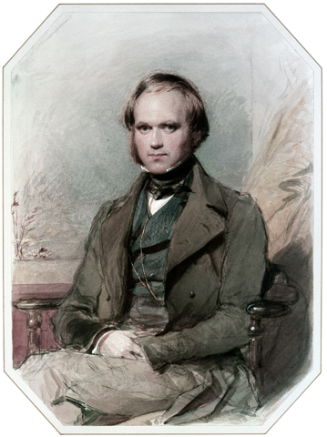
Captain of the boat couldn't talk to anyone else aboard because they were too low-class. So he brought Darwin as a gentleman of the higher strata to talk to.
Darwin's book On the Origin of Species is supposed to be quite fun. The first edition particularly didn't have the degree of vagueness ("if, maybe, maybe not") that was later added.